The Illustrated Conformer
From sound waves to FastConformer, Cohere Transcribe, and Parakeet
Posted on September 18, 2026
I’ve been thinking about speech recognition again. Not because I need another voice project (I already made one in an earlier post), but because modern ASR model cards now contain a small alphabet soup: CTC, RNN-T, TDT, FastConformer, attention encoder-decoder. I wanted to understand which bits were actually the same model, and which bits were merely sharing a family photograph.
That curiosity sent me back to Jay Alammar’s wonderful The Illustrated Transformer. It showed me how a good diagram can make a difficult architecture feel like a route through a city rather than a box of mysterious arrows. This post is my own visual walk through speech recognition, explicitly inspired by that approach. The writing and all the diagrams here are original; I haven’t copied Jay’s composition or artwork.
# Starting with a sentence, not a definition
Let’s use one utterance throughout:
“The small green boat is leaving.”
A microphone doesn’t hand an encoder that sentence. It hands over a changing pressure wave. We sample that wave, slice it into short overlapping windows, and turn each window into a vector describing energy at different frequencies. The model’s job is to turn a long sequence of those vectors into text, while coping with accents, noise, pauses, and the fact that people don’t politely leave spaces between sounds.
The first useful distinction is between an encoder and a decoder. The encoder turns audio frames into contextual representations. The decoder turns those representations into a transcript. FastConformer describes the encoder; CTC, RNN-T, TDT, and autoregressive decoding describe different routes from its output to text.

# From pressure waves to frames
The original Conformer paper uses 80-channel log-Mel filterbanks. The Mel part places frequency bands on a perceptual rather than linear scale: it keeps finer resolution at lower frequencies and groups higher frequencies more coarsely, roughly following human hearing. It does not simply remove everything outside the speech range. Instead, it builds a useful perceptual bias into the input, giving the model a more speech-friendly representation to learn from. The log part also compresses large differences in energy.
In the paper’s recipe, a 25 millisecond window is shifted by 10 milliseconds at a time. Each new slice therefore overlaps the previous one: speech information doesn’t fall into a crack between two frames. A two-second recording produces roughly 200 time steps before subsampling.
You can think of each frame as a tiny vertical strip: low frequencies at the bottom, high frequencies at the top, and brighter values where more energy was present. It isn’t a photograph of sound, and it isn’t yet a token sequence. It is a reasonably compact, machine-friendly description of what the microphone heard.
The Conformer encoder begins with convolutional subsampling. In the original setup, two strided two-dimensional convolution stages reduce the time and frequency grids, amounting to 4x subsampling. That makes later attention cheaper, although it also means the network has to preserve useful information while shrinking the view. The result is fed through a stack of Conformer blocks.

# The block with two half steps
The clever bit of the original Conformer is that it combines two kinds of context. Multi-head self-attention can connect distant moments: “boat” can influence the interpretation of a later sound even when many frames sit between them. Convolution is local: it is good at nearby patterns such as transitions between phonemes. Speech needs both the wide map and the close-up.
An exact Conformer block, in order, is:
- a feed-forward network whose output is multiplied by one half before residual addition;
- relative-position multi-head self-attention with a residual connection;
- a convolution module with a residual connection;
- a second feed-forward network whose output is multiplied by one half before residual addition; and
- a final LayerNorm.
The first and last feed-forward contributions are sometimes written as 1/2 FFN. This does not mean two smaller FFNs. They are regular FFNs whose outputs are multiplied by one half before they are added to the unscaled residual stream. This is the Macaron-style arrangement: the attention and convolution sit between two half steps of feed-forward processing.
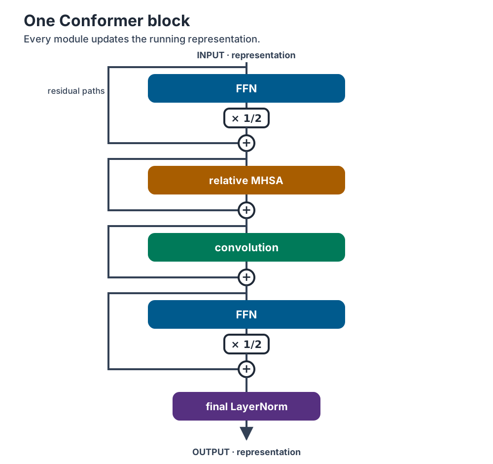
It helps to read the block as an update to a running representation. The first FFN nudges it, attention shares information across the utterance, convolution polishes nearby timing and sound patterns, and the second FFN nudges it again. Residual paths let each module specialise without having to rebuild the whole representation from scratch. LayerNorm at the end stabilises what gets passed to the next block.
# A closer look at the convolution module
The convolution branch is not just “put a CNN somewhere in the middle”. The paper’s module follows a particular sequence:
- LayerNorm;
- a pointwise convolution;
- a GLU (gated linear unit);
- a one-dimensional depthwise convolution;
- BatchNorm;
- Swish (also commonly called SiLU);
- another pointwise convolution; and
- dropout before the residual addition.
Suppose the input has T time positions and d feature channels. The first pointwise convolution is a one-dimensional convolution with kernel size 1, so it treats each time position independently. At position t, it applies the same learned linear projection:
$$ y_t = W x_t + b, \qquad W \in \mathbb{R}^{2d \times d}. $$
Each of the 2d outputs is a different weighted sum of all d inputs. If d = 3, this is simply a 6 × 3 matrix producing six combinations from three values. That is what “mixing” means here. It does not add time positions or create twice as much independent information; it creates a wider intermediate representation with shape T × 2d.
The GLU splits those 2d channels into two d-wide halves, uses one half as gates for the other, and returns T × d. The depthwise convolution then gives every channel its own temporal kernel, so it looks across nearby time positions without mixing channels. In the original Conformer paper, each kernel has length 32. With padding, the time length is preserved, making this another T × d → T × d operation; its kernel weights have shape d × 1 × 32.
Batch normalisation and Swish prepare the signal for a final kernel-1 pointwise convolution, which applies a learned d × d projection while keeping the shape at T × d.
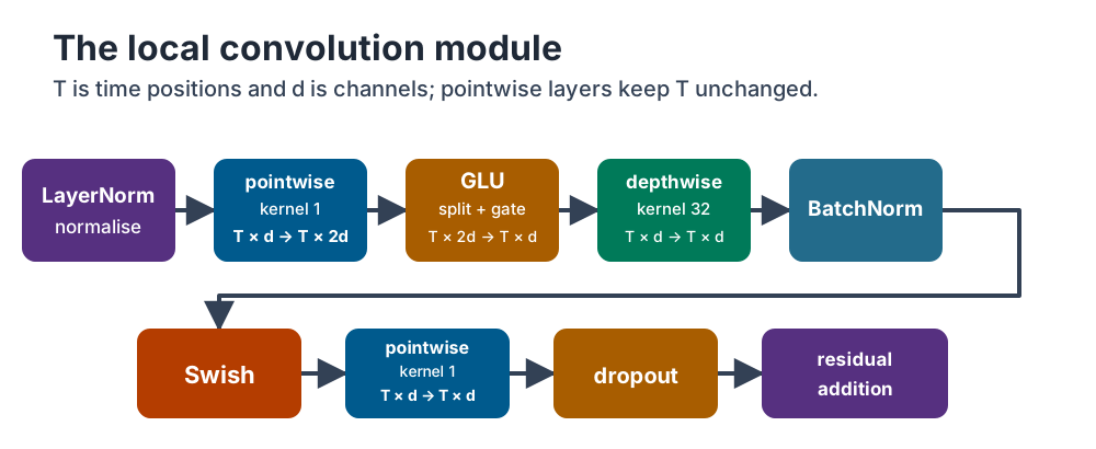
Attention connects distant positions, while convolution focuses on nearby patterns. Together they give the encoder complementary ways to organise sound.
# One Conformer system, not just one block
The original paper pairs its Conformer encoder with an RNN-Transducer (RNN-T). Its one-layer LSTM prediction network reads the text tokens already emitted. If the current transcript is “The small green”, that token sequence is the history. The prediction network turns it into a vector, and the joint network combines that vector with the encoder’s current acoustic representation to predict the next token or a blank.
RNN-T works incrementally: it can emit a token at the current acoustic position or emit a blank and advance through the audio. That makes it a natural streaming decoder. The original Conformer encoder, however, uses full-context attention and waits for future audio. Streaming Conformer variants restrict attention to available context. Pair one of those encoders with RNN-T, and the complete system can stream.
# FastConformer: make the front door narrower
FastConformer retains the Conformer block topology. Its main speed idea is earlier, in the front end. The FastConformer paper changes 4x subsampling to 8x subsampling: three 2x stages make the sequence entering the encoder one eighth as long as the original feature sequence, rather than one quarter as long. In other words, the encoder receives half as many time positions as in the baseline. The second and third subsampling layers use depthwise-separable convolution.
FastConformer also changes the depthwise convolution inside every Conformer block. Its Conformer-RNN-T baseline uses kernel size 31, while FastConformer reduces it to 9. This is separate from the new subsampling front end; the block topology stays the same. The original Conformer paper used 32 rather than 31, so these numbers describe slightly different starting implementations.
“8x” means one-eighth the sequence length, not “eight times faster”. The shorter sequence gives every later attention layer fewer positions to process.

The paper also studies limited-context attention. Each position sees a local window, while a global token carries information across the whole utterance. Over T positions with a window of width w, this reduces attention’s pairwise work from roughly T² to Tw.
On an NVIDIA A100 80 GB GPU with batch size 128 and 20-second clips, the paper measures encoder throughput increasing from 169 to 467 samples per second. That is a 2.8x encoder speed improvement while maintaining accuracy. In a separate batch-1 memory test, limited-context attention lets the encoder process 11.25 hours of audio at once on one A100.
# Decoders: four ways out of the encoder
Now we can separate the decoder choice from the encoder. The miniature map below shows four common routes from encoder representations to text.
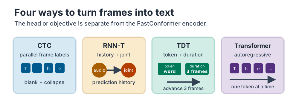
CTC (Connectionist Temporal Classification) assigns each frame a label or blank in parallel, then collapses repeats and blanks into text. The original paper is Graves et al. (2006).
RNN-T uses the tokens already emitted as its history. The prediction network encodes that history, and the joint network combines it with the current encoder representation to choose a token or blank. With a streaming Conformer variant, this can happen while the audio arrives. The original RNN-T paper is Graves (2012).
TDT, or Token-and-Duration Transducer, extends RNN-T by predicting both a token and a duration. The duration tells the decoder how many acoustic frames it can skip before the next decision. The primary reference is the TDT paper.
Finally, an autoregressive Transformer decoder emits one token at a time, using its previous tokens as history. Pair it with a Conformer encoder and you get the same broad encoder-decoder layout as Whisper, but with Conformer blocks in the encoder instead of Transformer blocks.
| Route | Predicts | Shape |
|---|---|---|
| CTC | Label or blank per frame | Parallel scores, then collapse |
| RNN-T | Token or blank plus history | Streaming-friendly with suitable encoder |
| TDT | Token and duration | Can skip frames |
| Transformer | Next token from history | Rich context, serial generation |
# How does this compare with Whisper and wav2vec 2.0?
Whisper is easiest to understand as a variation on the architecture we have already built. Start with a Conformer encoder and attach an autoregressive Transformer decoder. Then replace the Conformer blocks in the encoder with standard Transformer blocks. Whisper’s fixed front end first converts waveform samples into a log-Mel spectrogram.
Wav2vec 2.0 looks like the CTC version of the same swap. It reads waveform samples directly with a learned convolutional front end, uses standard Transformer blocks in the encoder, and applies a linear CTC head. Its opening convolutions learn the audio representation and shorten the sequence before the Transformer encoder.
# FastConformer in practice: Cohere and Parakeet
Cohere Transcribe combines a FastConformer encoder with an autoregressive Transformer decoder. It follows the same broad encoder-decoder pattern as Whisper, but uses FastConformer blocks rather than Transformer blocks in the encoder.
NVIDIA’s recent Parakeet collection keeps the FastConformer encoder and varies what comes after it. Its models use CTC, RNN-T, TDT, and hybrid combinations of those decoders. Together, Cohere and Parakeet show the main point: FastConformer describes the encoder, while the route from encoder output to text can change.

# Following the sentence through
Let’s return to “The small green boat is leaving.” After filterbanks and subsampling, the encoder sees a shorter sequence whose vectors contain both local acoustic detail and wider context. A CTC head may place distributions over repeated frame positions and blanks, eventually collapsing them into words. An RNN-T head may emit “The”, then use prediction history while consuming more encoder steps. A TDT head can decide that a stretch of frames carries no new token and jump over it. An autoregressive Transformer can keep producing the transcript one token at a time from its decoder history.
All four routes can transcribe the same utterance, but they align and produce the text in different ways. The encoder prepares the audio representation; the decoder determines the route to the final transcript.