Using Uncertainty to Monitor ML Models

In recent times, attention has started to shift from building machine learning models to deploying and maintaining them, which led to the growing interest for ML Ops. A crucial component in maintaining an ML model is monitoring: how do you know when it is time to retrain your model in production - when can you no longer trust its predictions? In our new paper, accepted at the AAAI 2023 conference, Carlos Mougan and I present a novel way to monitor models using uncertainty estimation methods, as well as improving the current state-of-the-art within uncertainty estimation.

• Link to paper
• Link to uncertainty estimation Python package
• Link to model monitoring experiments code

Here is our abstract:

Monitoring machine learning models once they are deployed is challenging. It is even more challenging to decide when to retrain models in real-case scenarios when labeled data is beyond reach, and monitoring performance metrics becomes unfeasible. In this work, we use non-parametric bootstrapped uncertainty estimates and SHAP values to provide explainable uncertainty estimation as a technique that aims to monitor the deterioration of machine learning models in deployment environments, as well as determine the source of model deterioration when target labels are not available. Classical methods are purely aimed at detecting distribution shift, which can lead to false positives in the sense that the model has not deteriorated despite a shift in the data distribution. To estimate model uncertainty we construct prediction intervals using a novel bootstrap method, which improves upon the work of Kumar and Srivastava (2012). We show that both our model deterioration detection system as well as our uncertainty estimation method achieve better performance than the current state-of-the-art. Finally, we use explainable AI techniques to gain an understanding of the drivers of model deterioration. We release an open source Python package, doubt, which implements our proposed methods, as well as the code used to reproduce our experiments.

This post is part of my series on quantifying uncertainty:

1. Confidence intervals
2. Parametric prediction intervals
3. Bootstrap prediction intervals
4. Quantile regression
5. Quantile regression forests
6. Doubt
7. Monitoring with uncertainty

# Uncertainty Estimation of ML Models

The uncertainty method introduced in the paper closely resembles the method I described in my previous post on boostrap prediction intervals and is implemented in the Python package doubt, which is described in this post. The basic idea is to estimate and combine several sources of variation in our ML predictions, and create prediction intervals from the combination of all these sources.

Firstly, we want to estimate how much the model depends on specific samples of our training set. We do this by sampling parts of the dataset, fitting the model on each of them in turn, and measuring how different the predictions of the resulting models are. Secondly, our models might have an inherent bias, meaning that it will never be able to fully approximate the underlying data distribution, no matter how much data we throw at it. This can for instance happen if we use a linear regression model to estimate non-linear data. The model will forever try to approximate the data distribution with a line (or higher-dimensional variants thereof), no matter how much of the underlying data distribution is sampled. Lastly, we want to estimate the noise that the model inherently has, again no matter how much data we throw at it.

We approximate all of these sources of noise using bootstrapping, and from these sources we can produce very accurate prediction intervals. This is an example from a previous blog post of a prediction interval generated by our method with a decision tree regressor as model, on synthetic data:

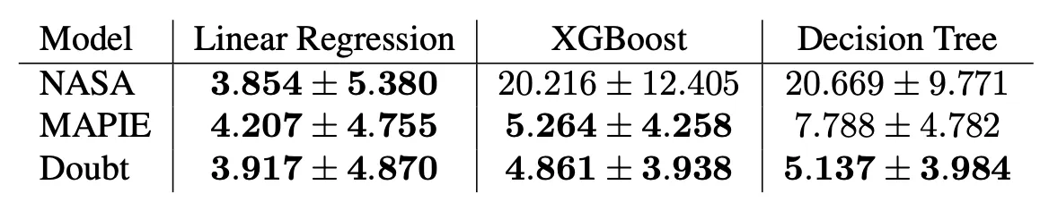
This method beats the current state-of-the-art methods from Kumar and Srivastava (2012) and Barber et al. (2021), as shown in the following table, which are based on nine datasets from the UCI repository, and we have marked the best results in bold, along with other methods which are not statistically different from the best result. Here Doubt refers to our method, NASA is the method introduced in Kumar and Srivastava (2012) and MAPIE the method from Barber et al. (2021). Lower is better:

# Monitoring ML Models using Uncertainty

With an uncertainty measure it turns out that we can monitor a model quite easily. We first compute the prediction intervals, and simply measure how wide the interval is. This represents how uncertain the model is in its predictions, and we show that this measure is highly correlated with the model’s actual prediction error.

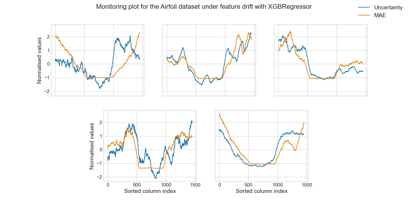
We conducted an experiment where we, for each feature of a given dataset, we gradually shifted that feature and recorded both the model error under this distribution shift, along with its associated uncertainty values. We see a clear correction between the model’s mean absolute error (MAE) and our uncertainty values, for each of the five features in the dataset:

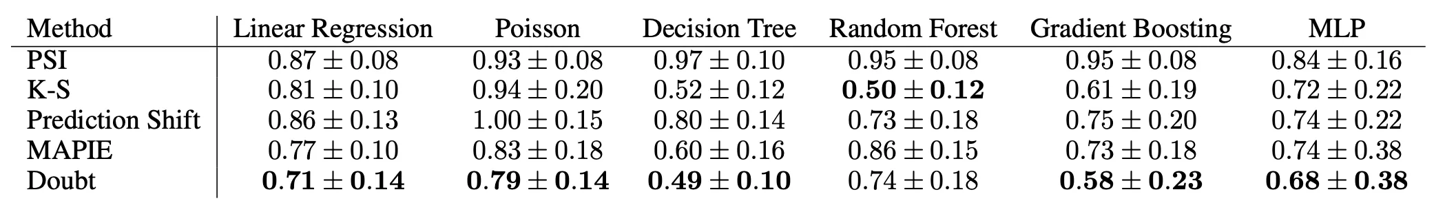
This method is of course compatible with any uncertainty estimation method, but we further show that our uncertainty method also provides significantly better monitoring performance. Here we compared our performance to both the MAPIE uncertainty estimation method, as well as several other classical statistical methods which are used to monitor models. In the following table we see that our method provides more accurate estimation of the model’s deterioration, except for random forests. Here Doubt is our method, and lower is better:

# Detecting the Source of Deterioration

One thing is to detect when a model is deteriorating, but sometimes we might want to know how it is deteriorating. This could for instance be due to a shift in one or more variables, the knowledge of which are the sources of model deterioration might be useful in its own right.

To account for the reasons of model deterioration, we fitted a separate model on the uncertainty values (i.e., the inputs to this model is the shifted feature values, and the outputs are estimated uncertainties). We proceeded to compute SHAP values (or any other xAI technique) of this separate model, which then shows which features of the dataset contributes the most to an increased uncertainty.

To test this approach, and compare it to competing methods, we took one of our datasets and shifted two features which were the most correlated with the target variable, GrLivArea and TotalBsmtSF, as well as introducing a random variable and shifting that as well. We thus want the model to identify the first two features, but disregard the random one, as it being shifted does not affect the model performance at all. Here are the results:

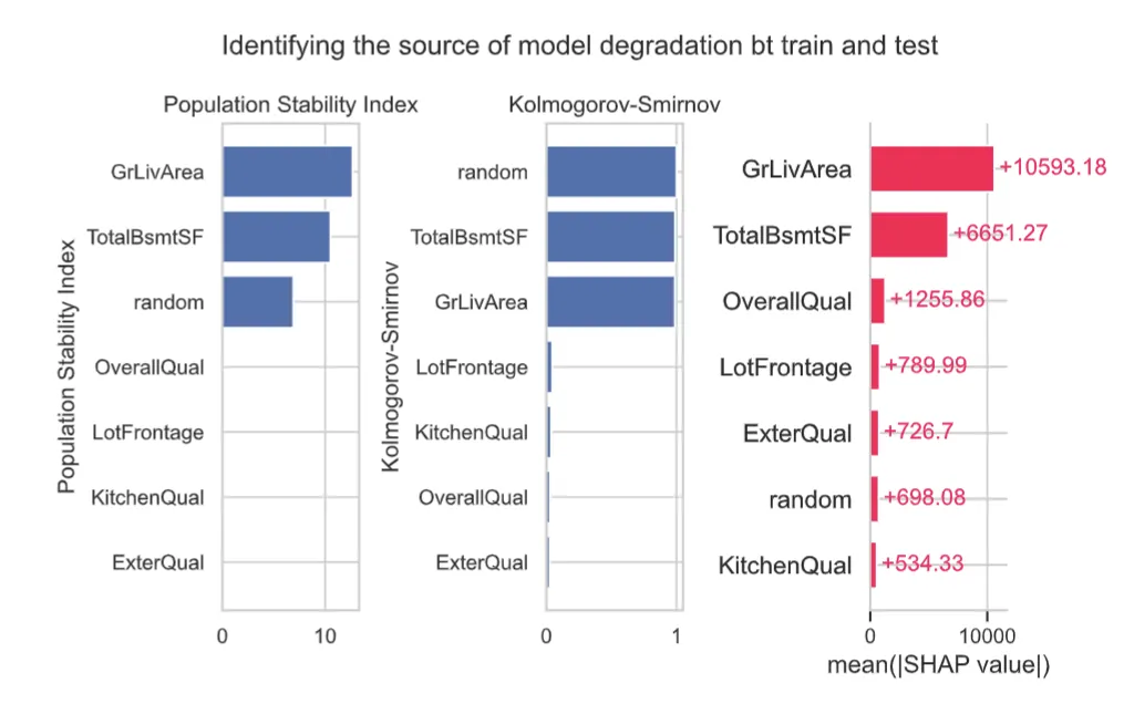
We see that our SHAP approach correctly identifies the first two features, as well as assigning a low value to the shifted random feature. The other two methods also identifies the first two features, but they attribute a substantial portion of the deterioration to the random feature.

Of course, this does not directly show the reason for the deterioration, but instead just the uncertainty proxy - but we can see this as an educated guess about which features might be the cause of the degradation in model performance.

A snippet of code that might help to reproduce and understand this paper contribution:

from sklearn.linear_model import LinearRegression
from doubt import Boot
import numpy as np

# Generate normal-distributed random data
x1 = np.random.normal(1, 0.1, size=10000)
x2 = np.random.normal(1, 0.1, size=10000)
x3 = np.random.normal(1, 0.1, size=10000)

# Create a synthetic dataset with the random data, of shape (1, 3)
X = np.array([x1, x2, x3]).T

# Create out-of-distribution data by shifting the first feature by 5
X_ood = np.array([x1 + 5, x2, x3]).T

# Create the target variable, which depends non-linearly on `x1`, linearly on `x2`, and does not depend on `x3` at all
y = x1 ** 2 + x2 + np.random.normal(0, 0.01, 10000)

# Create linear regression model with uncertainty estimation support, using our `Boot` wrapper class
clf = Boot(LinearRegression())

# Fit the model to the data
clf = clf.fit(X, y)

# Compute predictions along with prediction intervals on the out-of-distribution data
preds, intervals = clf.predict(X_ood, uncertainty=0.05)

# Compute the uncertainty, being the width of the prediction intervals
unc = intervals[:, 1] - intervals[:, 0]

# As for explaining where the uncertainty comes from, we fit a new linear regression model
# on the out-of-distribution data, which attempts to predict the uncertainties
m = LinearRegression().fit(X_ood, unc)

# Print out the coefficients of the second model, which corresponds to the SHAP values.
# We see that it puts no importance on any of the variables, as they are merely random
np.round(m.coef_, decimals=2)
#[ 0.01,  0.  , -0.  ]

# Citing Our Paper

@inproceedings{mougannielsen2023monitoring,
  title={Monitoring Model Deterioration with Explainable Uncertainty Estimation via Non-parametric Bootstrap},
  author={Mougan, Carlos and Smart, Dan Saattrup},
  booktitle={AAAI Conference on Artificial Intelligence},
  year={2023}
}